Over the last four weeks, we have discussed different strategies to calculate the number of shrimp in our pond in different periods of time; that is, we have been trying to estimate the survival in our pond. Although survival is one key element in estimating biomass (and possibly the most challenging one to obtain), we also need one more data point to get our biomass estimate: individual weight.
As we mentioned in our first post of this series, capturing the individual weight of all the shrimp in our pond is nearly impossible. Furthermore, we would need to get this information on periodic bases (at least once per week), so capturing, weighing, and separating each shrimp is not the way to do this. Also, let’s remember that we are already doing some data capturing with our survival estimation, so we better get the best out of the time and effort we are investing in gathering data.
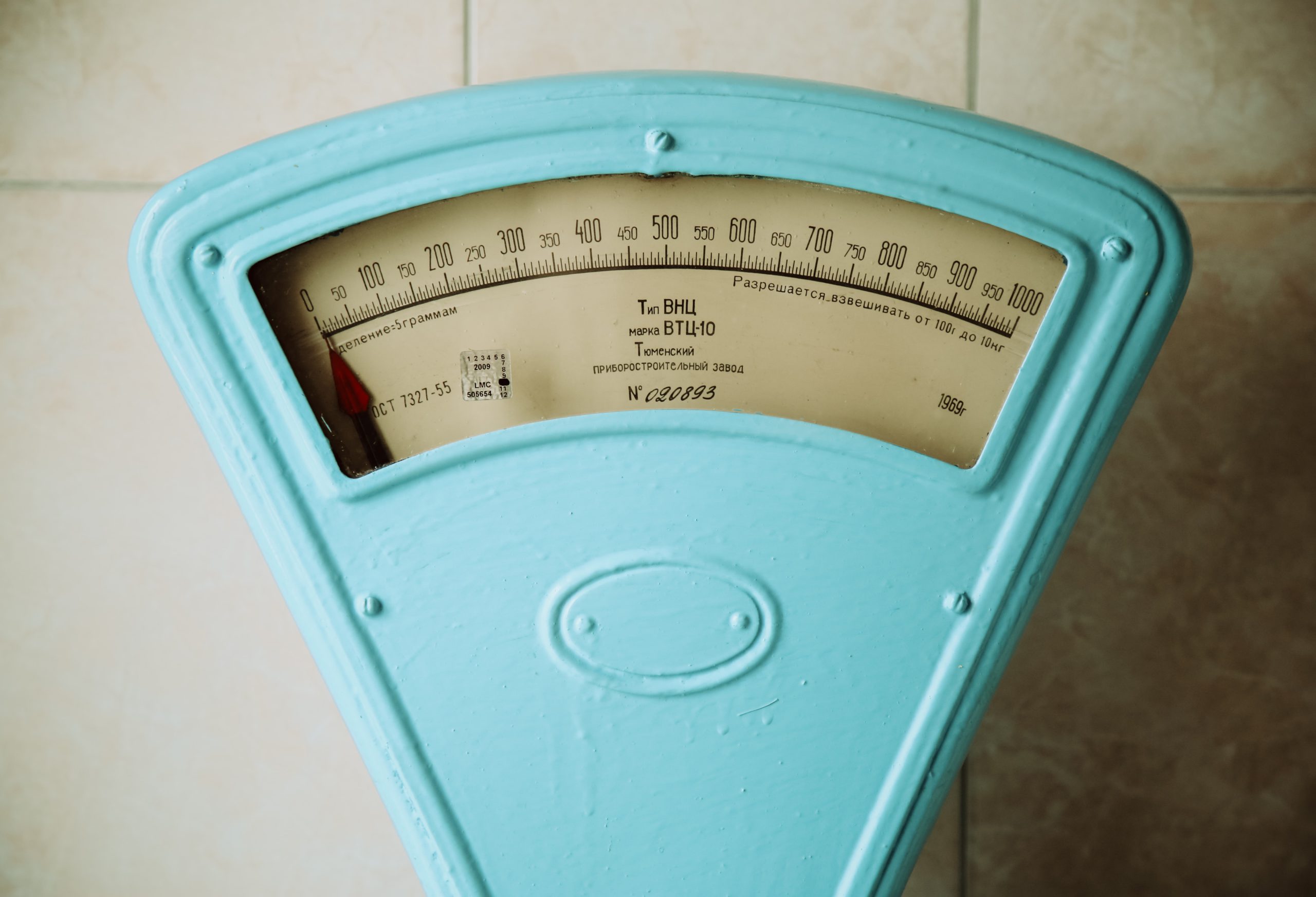
When estimating survival in our pond through the sampling method, we used a net to capture and count the shrimp in our pond. To optimize this effort, we can weigh what we caught before counting and divide it by the shrimp count we got for survival estimation; this way, we will calculate what is known as average individual weight.
An example of how this could work is following the next steps:
1.- fill a bucket or a tray with pond water, put it on a scale, and tare its weight.
2.- Throw the net in the pond as uniformly as possible.
3.- Retrieve the net with the catch and put the caught shrimp inside the bucket or tray.
4.- Capture the weight of the total catch.
5.- Count the number of shrimp caught.
6.- Divide the total weight of the caught shrimp by the total number of shrimp caught.
With this simple method, we will get two extremely valuable insights: the survival per unit of area (as we saw in the second post of this series) and the individual average weight. Remember that we need to estimate and obtain a significant sample size for these values to be a significant representation of our pond’s population.
Now we know not only the number of shrimp in our pond but also the individual weight (which will determine the selling price), and we can estimate the biomass.
Biomass will simply be the number of shrimp in our pond multiplied by the average individual weight of our shrimp. Obviously, there will be a certain error in our estimation associated with size heterogeneity and pond population, but at least we have a significant and approximate value now.
Forecasting
Just as we explained in our last post concerning survival, we can also model our shrimp’s growth. Once we have a couple of production cycle’s growth data, we can model the expected average weight of our shrimp. For this, there are several functions and variations. One can model intrinsic growth rate and from that extrapolate to individual weight, or we can directly model weight using variations of famous functions like von Bertalanffy’s or Gopertz’s curves.
Once we select a model, we can fit the curves using our historical data, just as we did in our previous post to determine survival; this way, the models will be tailored to our system.
Modeling biomass will let us make better decisions regarding our farm: from the amount of feed provided (which can be around 60 to 70% of our variable costs) to the best time to harvest (should I harvest smaller shrimp faster or bigger shrimp in a longer period?). In the end, a model will be a tool that we can use to improve the profits of our farm by optimizing processes.
The models can then be further sophisticated, accounting for size heterogeneity, changes in the growth rate associated with production density (linked with partial harvests), or even accounting for water quality indicators and their influence on biomass, such as the effects of temperature, oxygen, pH, salinity or ammonia on growth and survival. This sophistication will allow us to better understand our system, which can help us optimize the production through improved aeration methods or specific water exchange protocols.
Optimization is a very powerful tool to improve profit margins and increase a farm’s competitiveness; for this to be applied mathematically, modeling the farm’s production is a must, and although it might be complicated at first, it is undoubtedly an effort that is worth the investment.
