Estimating Biomass: Modeling Survival

As we have seen over the last couple of weeks, measuring the number of individuals in a shrimp pond is crucial but is also a difficult job. We need to estimate the sample size that will have significance for our measures, and, furthermore, we have to perform the samples, which consumes time and resources, but in the end, is a necessity.

Since this process is expensive and time-consuming, we must exploit the data gathered as much as possible to make the best of our investment. At first, it might seem like the only thing to do with this data is to know the population in our pond at that time, but once we have enough data gathered, there might be more we can do.

Over the following lines, we will talk a little more in-depth about how we can exploit our data to maximize its benefits instead of just storing the numbers in a computer or a file, never to be used again.

First, let us remember that we want to know the number of shrimp in our pond in order to estimate biomass, so we can know how much to feed and, maybe more importantly, how much we will harvest. This information is crucial to the farmer, not only to know our revenue at the end of the production cycle, but it also gives us an idea of how much can we leverage (that is, how big of a loan can we get), when is the best time to harvest, what is my production efficiency in terms of feed and energy, among other significant values. To get all this analysis, we need to be able to forecast, that is, predict the performance or the behavior of our survival. The main forecasting tool available is mathematical modeling.

Just as with the sample sizing, prediction models rest over statistics theory. Basically, we will create a model that follows a known survival path and then adjust the curve depending on the gathered data.

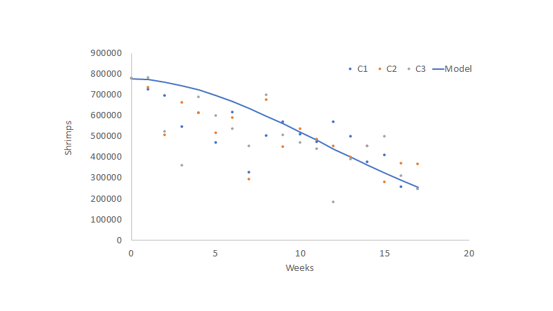
Let’s say we have been getting samples over the last three production cycles. We calculate the average survival for each week in each cycle and get a dot cloud.

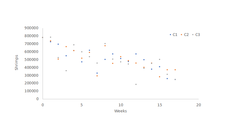
At first, it might be challenging to observe a pattern, but there are certain things we know about survival. First, we cannot have increased survival, meaning we can’t have more shrimp in our pond than what we initially seeded. Secondly, and in general, we can expect survival to decrease as time passes due to increased mortality in our system. Third, we know this mortality is not necessarily linear, meaning shrimp will die more during the first days of production, and then the population might stabilize, reducing the mortality rate. Finally, we can’t have a survival inferior to zero; therefore, we can’t have negative numbers in our final value.

With that simple bases, we can start thinking that our model follows an exponential distribution, exemplified in the figure below.

Now we only need to set the parameters so that our curve is adjusted to the observed data. For this, a very common model already developed fits very well with survival in most animal production situations.

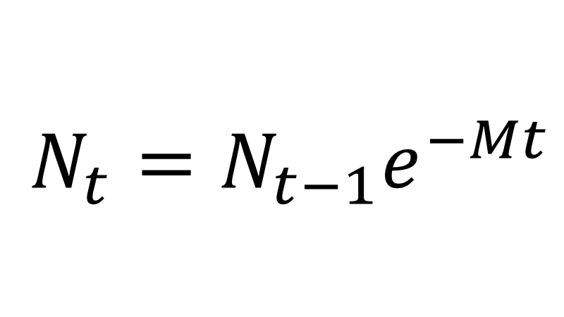
Where N_t is the number of shrimp present in time t, N_t-1 is the number of shrimp present in the previous period (i.e. the previous observation) e is Euler’s number, which is a constant, t is the time elapsed between observations, and M is the parameter that will help us fit our curve, also known as the instant mortality rate.

Once the model is calculated or incorporated into a spreadsheet with seed values for the unknown parameters (in this case, M=0.1), we get a first approach to how the data will behave.

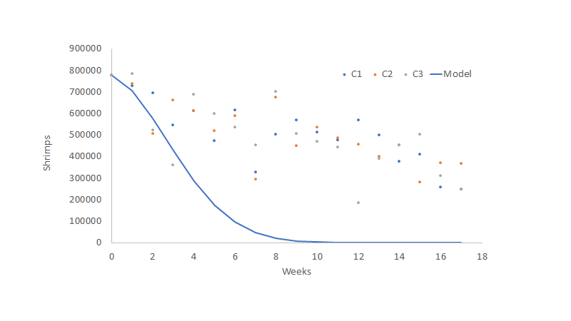
As we can see, the model does not fit our observations very well, so we need to fit our curve to the observations gathered (the data). Some software tools can help us get the parameter M, which is the one that helps us fits our curve. For example, we can use Excel, and its optimization tool included named “Solver”.

The process through which we obtain the value of M that better fits our data is called “parametrization”. There are several parametrization tools around, and each have they’re peculiarities and uses, but in this case, we’ll apply the most common one used for non-linear functions (such as the exponential function we are using), which is known as non-linear minimum squares.

As its name suggests, the idea behind minimum squares is to find the parameter that minimizes the sum of the squared difference between the model and the data points. In other words, this method lets us get a parameter that best fits the curve to the data points. Once that has been done, we can get a better fit for our model, as we can see in the figure below.

The main benefit of this method is its forecasting possibilities, which, combined with an individual growth model, can help us predict our production biomass, which will allow us to have better inventory control, increased commercialization power, an improved understanding of our optimum harvest time, better management of costs, and overall an enhanced control over the farm’s financial aspects.

Aside from the forecasting possibilities, the best thing about this survival estimation method is that under similar circumstances of density, temperature, infrastructure, etc. we only need to get the parameters once, and then we can use those same parameters in future estimations. That being said, if we should keep capturing survival data continuously on our farm, and thus we can use that data to estimate new parameters, which will help to keep the model optimum.

One of the main disadvantages of this method is its implementation complexity. Most often, the models’ difficulty shies the farmers away from their use. Fortunately, in the era of information and thanks to today’s computing power, we can implement these models and their parametrization automatically, leaving the complex calculus to the software and only using the outputs of the model to develop possible scenarios for our farm, optimizing several aspects of production and, in the end, maximizing the profitability of our farm.