Estimating Biomass: How do I get a significant sample size?

As described in our previous post, there are a few indirect ways to estimate the shrimp population in our pond to assess the biomass we produce. Over the following weeks, we will discuss in detail each one of the methods described in our previous post, as well as their pros and cons.

The first method we are discussing is the most common one, which consists in estimating the population through a series of samples. This method is very commonly used in biological sciences, particularly in ecology, especially when we want to estimate the population of a species in an ecological niche. One widespread use of this technique is applied in fisheries sciences. Since estimating the population of a species of fish in the sea is impossible to measure directly, scientists use indirect methods to estimate the biomass of each group of fish and establish the fishing quotas so that the natural stock of said fish is not depleted.

Following the same strategy, aquaculturists use similar sampling methods to estimate the biomass in a pond or a tank. As opposed to fisheries, shrimp farmers have more control over the area of study than fisheries scientists, which allows for a better estimation of the pond’s biomass.

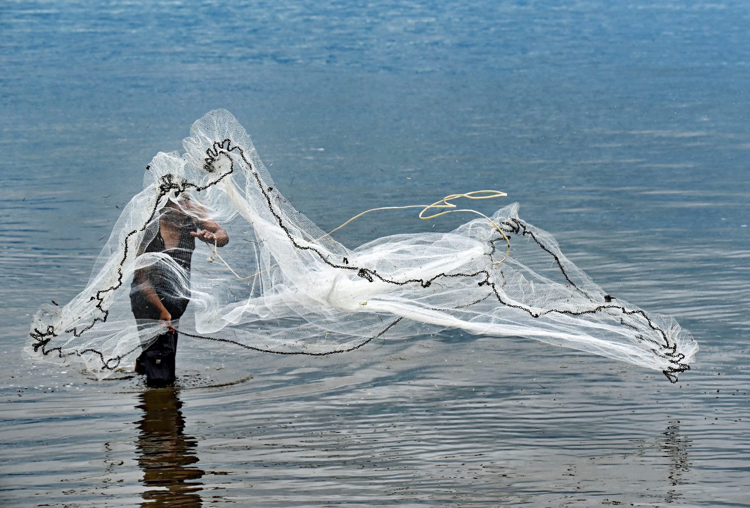
As described in our previous post, the method for estimation is quite simple. Farmers throw a net with a known diameter into the pond, then the net is extracted from the pond, and the population is counted, i.e., how many shrimp were caught in the net. With that information, a farmer can know the population in a particular area, and then he can extrapolate that value to the total area of the pond. Let’s do an example.

Say we have a one-hectare pond (that is 10,000 m²), and we want to know how many shrimp are in our pond. We are going to use a 1.13m diameter net, which is roughly equal to a 1m² area, to estimate our population. We throw the net in the pond covering perfectly our sample area (this is important, the net must be thrown correctly to cover the expected area), and extract 50 shrimp.

Since we have 50 shrimp in the net, that means we have 50 shrimp for each unit of area equal to the net’s surface, which is 1m²; therefore, we have a density of 50 shrimp per m²; if our pond is 10,000 m², then we only need to multiply the counted density by the area of the pond, which in this example would be equal to multiplying 50 times 10,000. Now we know how many shrimp we have in our pond, in this example, we have 500,000 shrimp in total.

Unfortunately, the previous example is not quite complete, and the reason is that we only did one sample for a 10,000 m² pond, meaning we sampled 0.01% of our total area; this would be enough if all shrimp were homogeneously distributed in the pond’s bottom., but we know this is not real since shrimp are distributed differently along the pond, with patches of higher population density and spaces of lower density. Let’s put a pin on that problem and continue with our example; we’ll cover this later in the text.

So, let us assume that 50 shrimp per m² is just what we expected to observe, but we go ahead and throw the net again in another part of the pond just to be sure the distribution is what we expected. When we collect the sample, we now count 200 shrimp in the net! Following the same reasoning as before, we assume we now have 2,000,000 shrimp in our pond! But that’s impossible, we think, since we seeded only 80 shrimp per m², and we just got a count of 50 shrimp in our previous sample, so it must be a mistake; therefore, we go ahead, move again to another part of the pond and throw the net, this time, there are no shrimp in our net, are they all gone? Do I have  0 shrimp in my pond then?

So what we decide to do now is an average. Since we found 50 shrimp the first time, 200 shrimp the second time, and 0 the third time, that means, on average, we have 50+200+0 divided by three samples; that is, we have 83 shrimp per m², and we only seeded 80… but we assume that the excess is probably due to an excess seed sent from the hatchery that was not accounted for in our seeding process, and we take that as our actual value.

The logic followed in our example is not entirely wrong. The sampling method (including the correct use of the net, covering its entire area; sampling different areas of the pond to avoid as much as possible sampling the same individuals; counting the individuals in each net throw; and calculating an average at the end) is correct and follows good practice and correct sample methodologies, but there is one critical mistake in our example, and that is the number of samples gathered, i.e., the number of times that the net was thrown.

Are three samples enough to significantly estimate the population in the pond? If not, how many should we do? Do we need to throw our net 10,000 times to cover all of the pond’s area? No, that would be inefficient, extraordinarily costly both in labor and in time, and, in the end, would not give 100% error-free population sampling (remember that each time the net is thrown, shrimp move in the pond, which means that, if we do 10,000 samples to cover all of the pond’s area, there is a substantial probability that we will count the same shrimp twice or more times and that we will miss some that are better swimmers) so covering the entire area 1m² at a time is not an option.

Should we increase the area of the net then? That is not necessarily a good idea; managing large nets is quite tricky. Remember that the net must be thrown correctly to cover the entire area, so it’s possible that we’ll throw more times a larger net in order to have a correct measure. And even if it were equally difficult, the statistical problem would persist as in we wouldn’t know how many times we need to throw the large net to get a significant sample size.

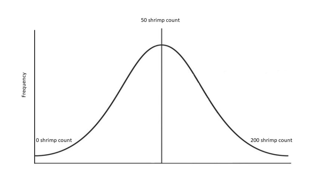
So, instead of covering the whole area, we need to rely on statistics to estimate the number of samples (or the sample size) that can be considered significant for our pond. But what is a significant sample size? In statistics, we consider a significant sample a sub-group representing the entire population or the full group, in this case, our pond. To calculate the number of throws that compose a significant sample size, we need to make one assumption, which is that the distribution of our population is normal; that is, it follows a bell-shaped distribution; which would mean that the frequency of the numbers obtained in each throw will follow this shape, in other words, and following our example, we would find more frequently values of 50 shrimp per throw than zero or 200.

Once this assumption is made, we need to determine the level of confidence in which we want our sample size to be and the desired level of error, meaning the greatest error our estimation can have to be considered valuable. For this, we’ll use absolute values of error (that is ± how many shrimp is acceptable to be under or overestimated by our method). Remember that the lower the desired error, the higher the number of samples will be needed.

In terms of confidence intervals, usually, levels of 95% are considered significant in most cases, and in that case, we can estimate the total error at approx. ±2 standard errors from our distribution. We’ll get back at this a little further in the text.

Once we have selected our precision and desired error levels, we can proceed to the error equations of the normal distribution:

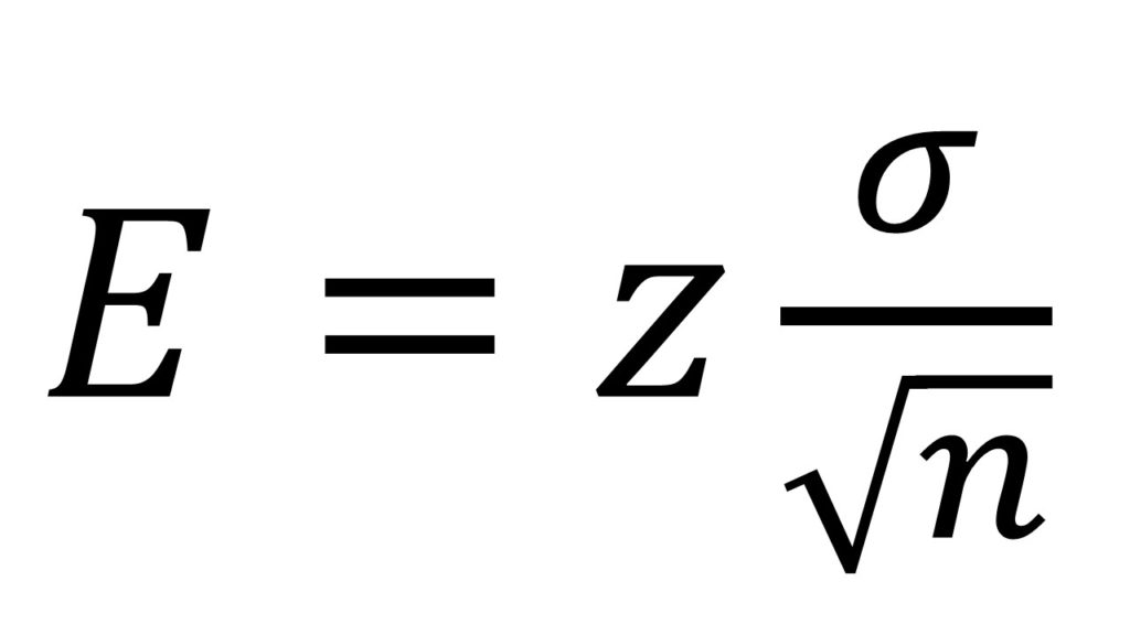
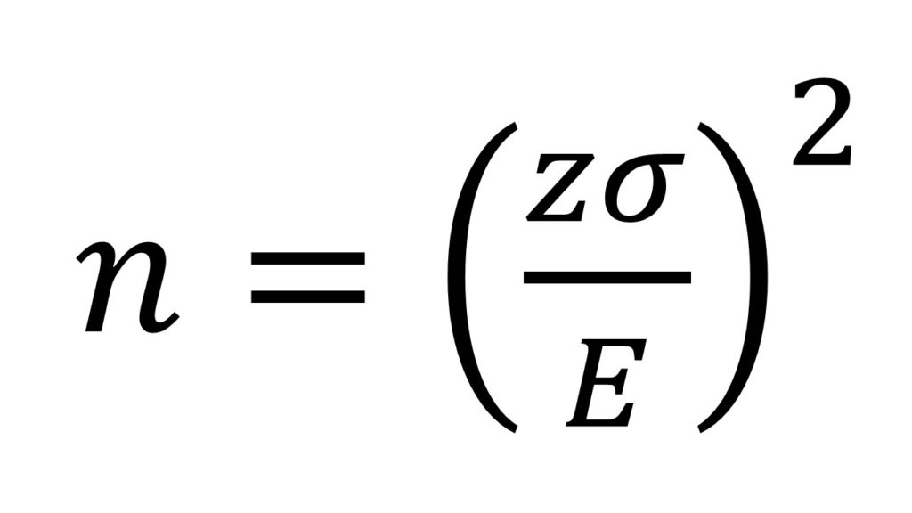
Where E is the desired error, z is the Student’s t value for n-1 degrees of freedom for the 1-α level of confidence (the tabulated value mentioned earlier, as I said, we’ll get back to this in a bit), σ is the standard deviation of the distribution, and n is the sample size needed to determine the mean, which is the value we want to know; therefore we need to rearrange the error formula to clear n, obtaining

We already selected our desired error and our confidence value of 95%, but still, a couple of numbers need to be obtained to get our answer. The first one is the standard deviation. We have two easy methods of obtaining a “first approach” for a standard deviation. The first one is through “guesswork”, which would mean including an expected number in there that we think (in our experience) will tell us the standard deviation of our sample. A more precise one is to estimate a “first approach” to the standard deviation through our first sample. We have three measures now (0, 50, and 200); now, we can calculate a standard deviation for those samples and use that as a seed value.

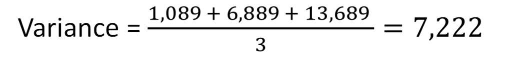
The standard deviation, or σ, is nothing but the square root of the variance. The variance is the average value of the sum of the squared difference between each observation and the average. In our example, the variance can be calculated as follows:

(50-83)² = 1,089

(0-83)² = 6,889

(200-83)² = 13,689

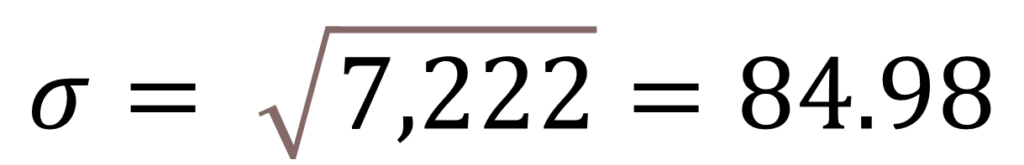
Since the standard deviation is the square root of the variance, then

Calculating the standard deviation is easy with small samples, but it can get tedious with larger samples, so we can use tools like excel or other computing software to do this.

Now we need to obtain our final value, Z. The problem here is that this tabulated value is dependent on the sample size (ironic, right?). Although there is an iterative method designed to obtain this value with trial and error without knowing the number of samples (n), it is much simpler to use an approximate value. Since we are aiming for a 95% confidence and we assume that the sample size is not too small, we can use the previously mentioned approximate value of 2 standard error deviations for z, meaning that, for this example, z=2.

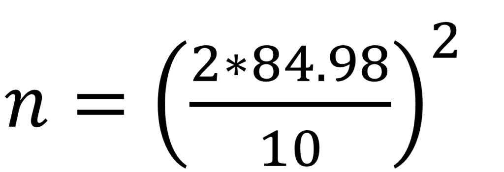
So, let us calculate our estimated sample size for this shrimp pond. We selected a desired error of 10 shrimp per m² with a 95% confidence interval (that is, z=2) and calculated our standard deviation, SD obtaining a value of 84.98. We then proceed to substitute in our equation

n = 288.89

We know that sampling 289 times each pond is impossible or at least extremely impractical, so there are a few things we can do to solve this. (1) get more samples to estimate our SD better, (2) reduce the confidence level we selected for our method, or (3) increase the desired error.

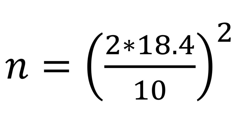
So let’s say, in our example, we detect that, according to our experience, the seed value for the SD is too high, and the enormous difference between our three samples seems to be the problem, so we go back to the pond and get a couple more measurements, ending up with an SD value of 18.4. We go ahead and try our equation again

n = 13.5

Now that sounds more like it. This means that to get a significant sample size and estimate our population with a 95% confidence and an error of 10 shrimp m², we need to throw the net 14 times.

As you can see, this is not necessarily a precise exercise. As often in statistics, there is a circular problem where you need to get data to estimate how much data you need, which can be confusing, but in the end, we can start with some data points and figure it out along the way. Suppose we already have historical information of samples. In that case, this is even easier since we can estimate our SD based on our previous data sets and then estimate our significant sample size.

Now we can do sampling and obtain statistically significant values to estimate the average number of shrimp in our pond. The steps are now similar to what we described in the first lines of our exercise, except now we get 14 net throws in the tank with the following results

Observation	Number of shrimp
1	28
2	50
3	55
4	38
5	66
6	50
7	47
8	71
9	82
10	35
11	45
12	55
13	19
14	20

On average, we have 47.21 shrimp per net throw, with a net area of 1m², meaning we have, on average, 47.21 ± 10 shrimp per m². Since our pond is 10,000 m², we can now say, within a 95% confidence interval, that we have a population of 472,100 ± 100,000 shrimp in the pond. We can increase precision by selecting the desired error in relative terms instead of absolute value, or if the absolute value of the desired error is reduced (say to ±1 shrimp per m²), but this means an increase in the samples needed (a tenfold increase in this case, so we would need 135 net throws per pond). In the end, we need to find a balance between operative feasibility in terms of the number of net throws per pond and the reliability of the results.

The main advantage of this method is that it’s simple (we only need a net with a known diameter), cheap (as long as we compromise with the number of samples), backed up by a very robust theory, and provides significant values. Furthermore, gathering this data can help us further in the future to develop mathematical models (which we will talk about in our next post). Also, we only need to estimate the significant sample size one time; once we know how many samples we need to have a significant value, this is true for all our future productions under the same conditions.

As a disadvantage, we can find that the error might be too large if we intend to have a reasonable amount of samples; otherwise, we would need a lot of human resources, eliminating the main advantage of this method, which is that it’s reasonably cheap. Something else to account for is the human component of the sampling method. It is important that the samples are always taken by the same person or that all the sample takers are equally trained in the method. This is significant since a deficient net throw would result in a different area, which could alter the results of the method