Shrimp farming basics: project viability and investment analysis

Over the last few weeks, we have been looking into some of the main aspects of shrimp farming, from feed and disease management to seeding and infrastructure. We have covered the essential elements that all farmers need to know and understand to have good productivity and improve their farm’s performance. In all cases, the mix of components that determine the success of a farm is composed of two main elements: knowledge and capital.

As you have seen all over the previous deliveries of this series, capital is the limiting factor when selecting infrastructure, feed, a management strategy for disease, aeration, recirculation, pumping, and so on. The correct selection of feed and equipment depends on how much I can spend on my farm and if that decision will positively impact future profits. In some cases, the selection of materials, pumps, tanks, personnel, feed, additives, and even management style can be counterintuitive. There is a generalized vision that the most expensive products will result in the best performance, but this is not always the case, as proven in previous installments.

Whether it is an expansion of our infrastructure, an investment in new technology, or the founding of a farm from scratch; in this final component of the series Shrimp Farming Basics, we will take a look into determining if an investment is worth it. For this, we’ll divide the evaluation into two different kinds of profitability evaluations, delivered in two papers. This first article will discuss the evaluation of an entirely new project and will introduce some economic indicators that are used to assess profitability. The second one is the evaluation of a new component in an already ongoing system, i.e. the expansion of our facilities, the inclusion of a new additive that improves health, or the automation of the farm, which will be presented in a second volume.

Viability of a new farm

Let us assume that we are an entrepreneur that would like to invest in shrimp aquaculture. We already know the design of the farm, the tanks, and materials that we’ll use, we have feed and seed providers, enough marine water for our system, the quality of said water is optimal for shrimp farming, and we estimated the equipment necessary for aeration and water exchange. With these estimations and models selected, we now want to know if it would be worth it to invest our money in shrimp farming or if we are better off buying some secure asset (like government bonds) and just getting those interests.

Before going into detail about how we’ll do this and how to have a sound cost structure, there is a critical concept that needs to be understood to fully grasp the idea of the economic indicators and why they work as they do, and that is the concept of the value of money in time or the “cost” of capital.

Basically, money has a cost and a value that will change as time passes. Money right now is more valuable than the same money given in, say, one year. This is mainly due to the possibility of using that capital for an investment that would pay me back a fraction of the input. For example, if I get one million dollars right now, I can go ahead and invest it at a 1.12% yield 12 month US bond so that I will get 12,000 USD in that same year; therefore, my 1 million USD is now worth 12 thousand USD more than at the beginning of the year.

With that concept in mind, economic indicators try to bring the value of money from the future to today’s value and see if our investment will be better than our alternative; for this, there is a critical economic concept known as opportunity cost.

The opportunity cost is understood as the return that you could get from your capital in another investment. In our example, the opportunity cost would be equal to the rate of return from the 12-month US national bonds (or 1.25%), but it could also be another business or a loan. Say, for example, that you can invest your money in the stock market and get a 6% yearly return of your capital in a medium-risk investment. Well, your opportunity cost would be equal to 6% yearly.

Now that the concept of opportunity cost is clear, we can present our first economic indicator, which will bring the future value of money to present, known as Net Present Value or NPV, described as

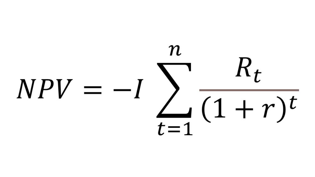
Where Rt is the total cash flow for year t, r is the opportunity cost, and I is the initial investment.

The formula might be intimidating, but it’s simple to understand and apply. The sigma symbol (∑) represents an addition, which means that we need to sum all our cash flows divided by the opportunity costs, from the first year (where t=1) up to the last year of our projection (where t=n, and n is the final year of the projection); usually, projects are evaluated to 5 or 10 years in the future. Since the initial investment is made in year 0, the opportunity cost doesn’t apply there, and its value is taken out from the addition of the cash flow. The estimated cash flow for each year will be the expected revenue minus the expected cost in each year, and that value is divided by one plus the opportunity cost, which is then raised to the year we are calculating. As we’ll see, cash flow will be smaller the longer in time they are evaluated; this is due to the value of money in time discussed earlier. Finally, we need to add all the estimated values, and we’ll get a number for the NPV.

The general rule says that if NPV is positive, the project design is better than our other investment (i.e. bonds or the stock market) and is, therefore, a good investment. On the other hand, if NPV is negative, our money would be better off in our second option.

Apart from the opportunity cost, the investment and the cash flow need to be very well researched and evaluated to produce a sound estimate and avoid future invisible costs that might make our project unprofitable.

As you may have deducted then, to have a reasonable estimation of the viability of our project, we need to estimate (or model) our future revenues. For this, we have to model how much money we can get from our farm and how much producing shrimp will cost.

Income is somewhat easy to estimate in shrimp farming. We only need to calculate our expected biomass at the end of the production cycle and multiply that by the expected selling price, hence getting our future revenue.

The costs can be a little more tricky to estimate, but we can generally divide our costs into two categories: fixed and variable.

Fixed costs are the ones that are not directly linked with the amount of production. Fixed costs need to be paid, whether you produce 0 or 10 million tons of shrimp. The main components of fixed costs are usually labor, rent, capital, and depreciation.

Capital costs are a special kind of fixed cost and are associated with the use of capital in one investment instead of another. We have already discussed capital costs earlier when talking about opportunity costs, but this is not the only component of capital costs. Other examples of capital costs are the initial investment or the capital structure of debt and equity.

Depreciation is another special kind of fixed cost that can sometimes be disregarded, causing future losses and, in extreme cases, even jeopardizing the sustainability of a farm. Depreciation consists of including into our cost structure the loss of value over time of all the equipment used and acquired for the farm. The continuous use of pumps, aerators, geomembranes, pipes, filters, etc. causes wear; this eventually makes it impossible to continue their use. Depreciation is then the cost of replacing the farm’s equipment. There are several ways to calculate depreciation, depending on the value of the equipment once it’s used (this is useful, for example, in the case of vehicles and other equipment with some resell value), or the need to replace it without any rescue value. A very simple method for its estimation consists of dividing the equipment’s worth by their expected years of service and adding that cost to the yearly fixed cost structure.

Application example

So all of this is interesting and everything, but how do we apply it? Well, let’s take a look at a very simple example. Keep in mind that several numbers and estimations are presented to understand the example better; in a real-life application, you must be as rigorous and specific as possible.

Say we can buy a 10 hectare land suitable for aquaculture for three thousand dollars per hectare. The land has a water well that can already provide the farm with ocean water, and the water has optimum levels of all the significant water quality indicators. We also hired a specialist to develop the infrastructure, and he came back with a list of the components we need, their cost, and expected service lifetime.

Component	Number	Unit Price	Total Cost	Lifetime (years)
Water pump	4	$   4,500.00	$   18,000.00	10
Filtration system	2	$   6,500.00	$   13,000.00	5
8m Circular tanks	108	$   1,450.00	$ 156,600.00	10
Aerators	20	$      665.00	$   13,300.00	10
Other equipment		$ 56,000.00	$   56,000.00	10
Total investment			$ 256,900.00

We now know the investment needed in infrastructure. We estimate that we can operate our farm with 30 workers who will provide feed, check the water quality parameters, monitor the animals, and attend to all farm’s needs. Furthermore, the engeineer charged us 15,000 USD for the project and presented what is needed to operate the farm as well as their unit costs.

	Unit cost	Units	Number	Total cost
IniTial investment
Aquaculture engeineer fees	$15,000.00	Project	1	$   15,000.00
Land	$   4,500.00	Ha	10	$   45,000.00
Infrastructure	$ 56,900.00	Project	1	$   56,900.00
				$ 316,900.00
Fixed costs (per year)
Labor	$      850.00	USD/month/worker	30	$ 306,000.00
Depreciation	$ 26,990.00	Total	1	$   26,990.00
Other				$   45,000.00
				$ 377,990.00
Variable costs (per year)
Feed	$ 800.00	ton	167	$ 401,241.60
Energy	$      0.04	kWh	463680	$   55,641.60
Seed	$      9.83	thousand	3715.2	$ 109,561.25
Other inputs			30000	$   90,000.00
Harvest labor	$    10.81	hour	16	$        518.88
				$ 656,963.33

With this project, he says, we will be able to produce 140 tons per year, and we estimate we can sell the product at a total of 8 USD per kg. So now we have all the information we need to estimate a cash flow and calculate the net present value to see if our project is viable.

Year	Cost	Revenue	Profit	Present Value
0	$    316,900.00		-$316,900.00	-$316,900.00
1	$ 1,034,953.33	$ 1,114,560.00	$   79,606.67	$   75,100.63
2	$ 1,034,953.33	$ 1,114,560.00	$   79,606.67	$   70,849.65
3	$ 1,034,953.33	$ 1,114,560.00	$   79,606.67	$   66,839.30
4	$ 1,034,953.33	$ 1,114,560.00	$   79,606.67	$   63,055.94
5	$ 1,034,953.33	$ 1,114,560.00	$   79,606.67	$   59,486.74
6	$ 1,034,953.33	$ 1,114,560.00	$   79,606.67	$   56,119.56
7	$ 1,034,953.33	$ 1,114,560.00	$   79,606.67	$   52,942.98
8	$ 1,034,953.33	$ 1,114,560.00	$   79,606.67	$   49,946.21
9	$ 1,034,953.33	$ 1,114,560.00	$   79,606.67	$   47,119.07
10	$ 1,034,953.33	$ 1,114,560.00	$   79,606.67	$   44,451.95

As we can see, the value of the future profits will be increasingly reduced the further in time we go; this is due to the opportunity cost of 6% that we estimated we would get from the stock market. Obviously, the higher the opportunity cost, the faster the present value is reduced.

Finally, we only need to sum all the values observed in the Present Value column to estimate the Net Present Value (NVP), which in this case is equal to  $ 269,012.04. Therefore, if we follow the NPV interpretation rule, and since the NPV is positive, we can determine that this is a profitable project and is better than our next better option.

There are other interesting indicators to assess our project and the investment on it, such as the internal rate of return (IRR) or the return on investment (ROI), but we will discuss them on another occasion.

Now we know if our investment in a shrimp farm is sound or if our money would be better off in another place; we know how to project and sell our project in order to get investments. In our next and final part of the series Shrimp Farming Basics, we will discuss how to evaluate the profitability of implementing new technologies (such as new feed brands, automation systems, or new management techniques) and do some basic benchmark analysis.

Note: Remember that the numbers given in the example are mere examples of how to make a projection and do not constitute actual values, nor should they be used to include in your own model. You must obtain as accurate numbers as possible according to the market and prices available in your region. The more precise your data are, the better your model results.